- Temp
- —
- °C
- TDS
- —
- g/L
- Turbidity
- —
- NTU
- Depth
- —
- m
- Sound speed
- —
- m/s
Environment-aware acoustic payload · Autonomous underwater vehicles
It's loud, layered,and never the same twice.
Not that the pulse noticed.
We're building sonar that reads the water first.
Adaptive Sonar
fixed-frequency sonar goes blind in water that moves
Sediment, temperature, salinity and depth all move the acoustic channel — and they move it during a survey, not between them. A pulse chosen on the deck is already the wrong pulse by the time it reaches the seabed.
solved on the payload itself
No cloud. No pairing. No network call. The optimiser, the physics and the DSP all run on the device, which is the only place they can run fast enough to matter.
How the payload adapts a sonar pulse to the water it is in
- Mode
- —
- fC
- —
- kHz
- B
- —
- kHz
- τ
- —
- ms
- Window
- —
- Resolution
- —
- mm
- Echo SNR two-way
- —
- dB
- Range
- —
- m
- Spreading
- —
- dB
- Absorption
- —
- dB
- Scattering
- —
- dB
- One-way TL
- —
- dB
- Echo SNR two-way
- —
- dB
TX
RX
SPEC
- SNR before compression
- —
- dB
- Processing gain
- —
- dB
- Sound speed
- —
- m/s
- α at band centre
- —
- dB/km
- Excess scattering
- —
- dB/km
- Margin required
- —
- dB
- Selected fC
- —
- kHz
FIXED
ADAPT
- PSLR
- —
- dB
- PSLR
- —
- dB
- Detection
- —
- Detection
- —
- DS18B20temperature
- TDS probeconductivity
- Opticalturbidity
- Pressuredepth
- Estimatec, α, excess
- DDSphase accum.
- DAC12-bit
- Recon.filter
- Driveranalog
- Transducerpressure
The medium is not constant.
Temperature, dissolved solids, suspended load and depth all decide how far sound carries. None of them hold still along a survey line.
One payload, one ping interval.
The payload measures the water, chooses a pulse, transmits it and compresses the return — all of it between one ping and the next, on the vehicle, with no link to the surface.
A pulse leaves the aperture.
A swept pulse, chosen for water this clear: the widest sweep the transducer will pass, because bandwidth is what buys range resolution.
The water changes.
Warmer, more conductive, and carrying sediment. The sound speed shifts, and the suspended load starts taking energy out of the pulse.
The loss follows it down.
Spreading is geometry and never changes. Absorption is the water itself. The third term — scattering off suspended matter — is the one that grows, and it grows fastest at the top of the band.
The water changed. The waveform did not.
The pulse that was correct an hour ago is still being transmitted. The echo it earns no longer clears the detection threshold at the range the mission asked for.
Measure the medium.
Temperature, conductivity as a salinity proxy, optical turbidity, and depth. Four numbers, read on the vehicle, in the water the pulse is about to cross.
Solve for the pulse.
Every candidate waveform is scored against the sonar equation for the water just measured. The widest sweep that still clears the threshold with margin wins. Nothing here is a lookup table.
Build it on the way out.
The chosen parameters go straight into the transmit chain — phase accumulator, converter, reconstruction, driver, transducer — and become a pressure wave.
The same water. A different pulse.
Nothing has been done to the sediment. The range is the range the mission wanted. The only thing that changed is what was transmitted into it.
The medium changes. The sonar adapts.
Matched filtering collapses the returning sweep into a single peak. What arrives buried under the noise leaves the filter as an arrival time.
One payload. Any water. Mission-ready.
The same hardware works a clear reef and a muddy estuary, because the waveform is a decision rather than a setting.
351 kHz
Top centre frequency
drops to 148 kHz as sediment loads
Modelled 470
Candidate waveforms scored
every tick, against the sonar equation
Measured 23.81 dB
Compression gain
time–bandwidth product 240.4
Calculated 13
Stages per ping interval
sample, solve, transmit, correlate
Measured 0
Network calls
no server, no pairing, no cloud
Measured Built to be questioned.
The system does not ask you to trust the number. It shows you where the number came from.
The model
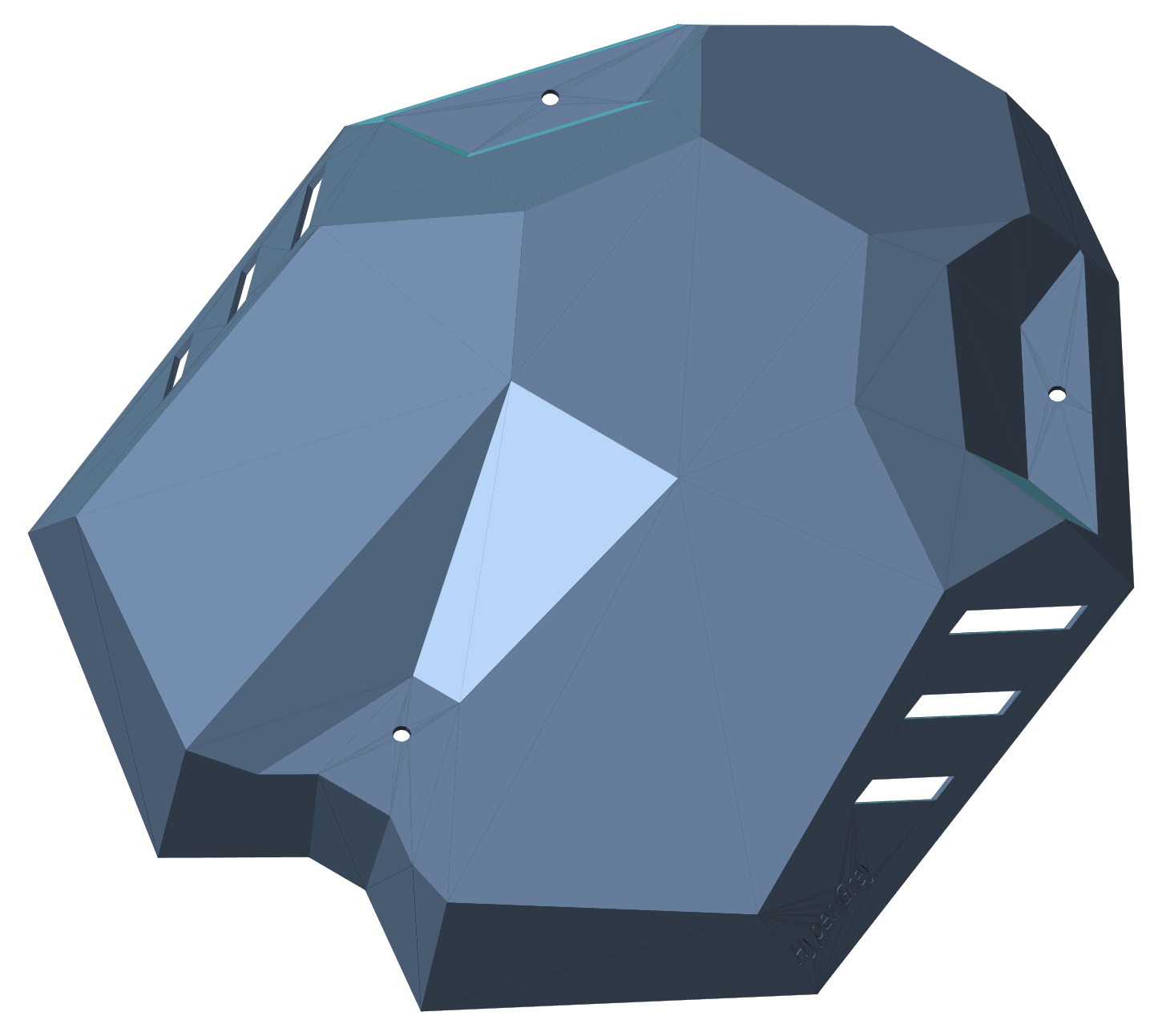
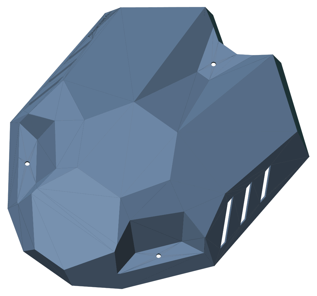
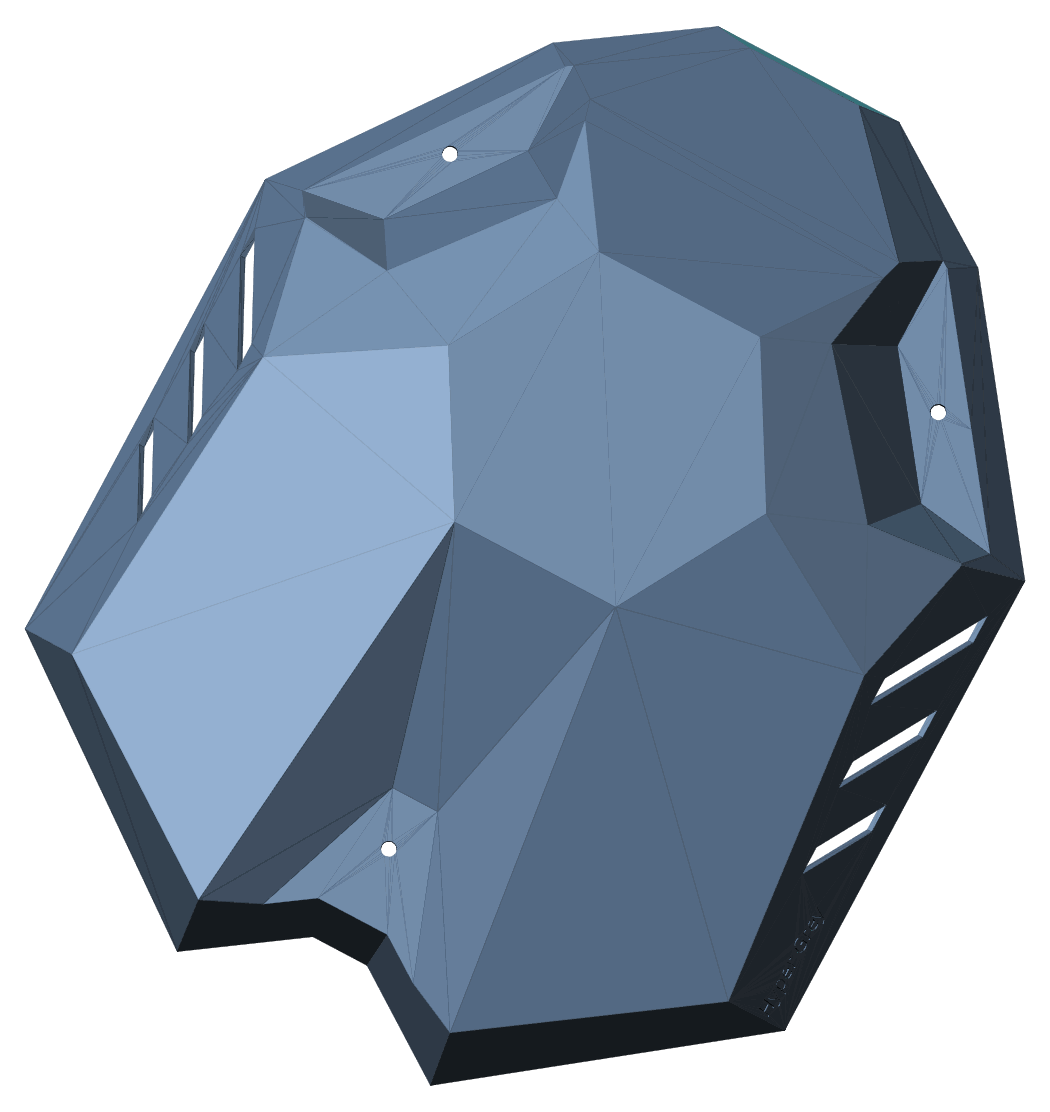
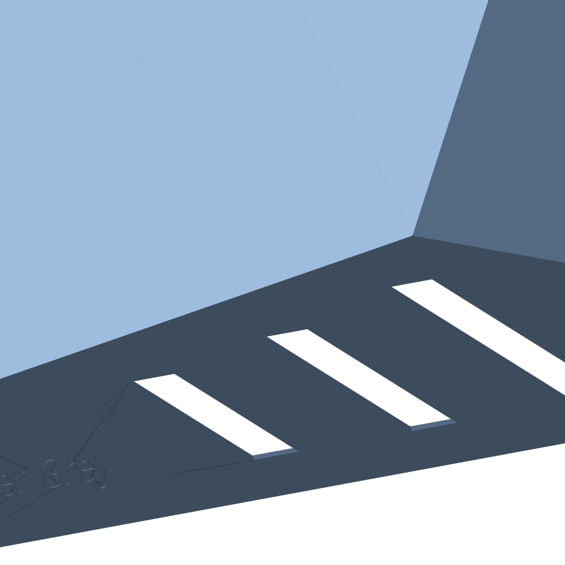
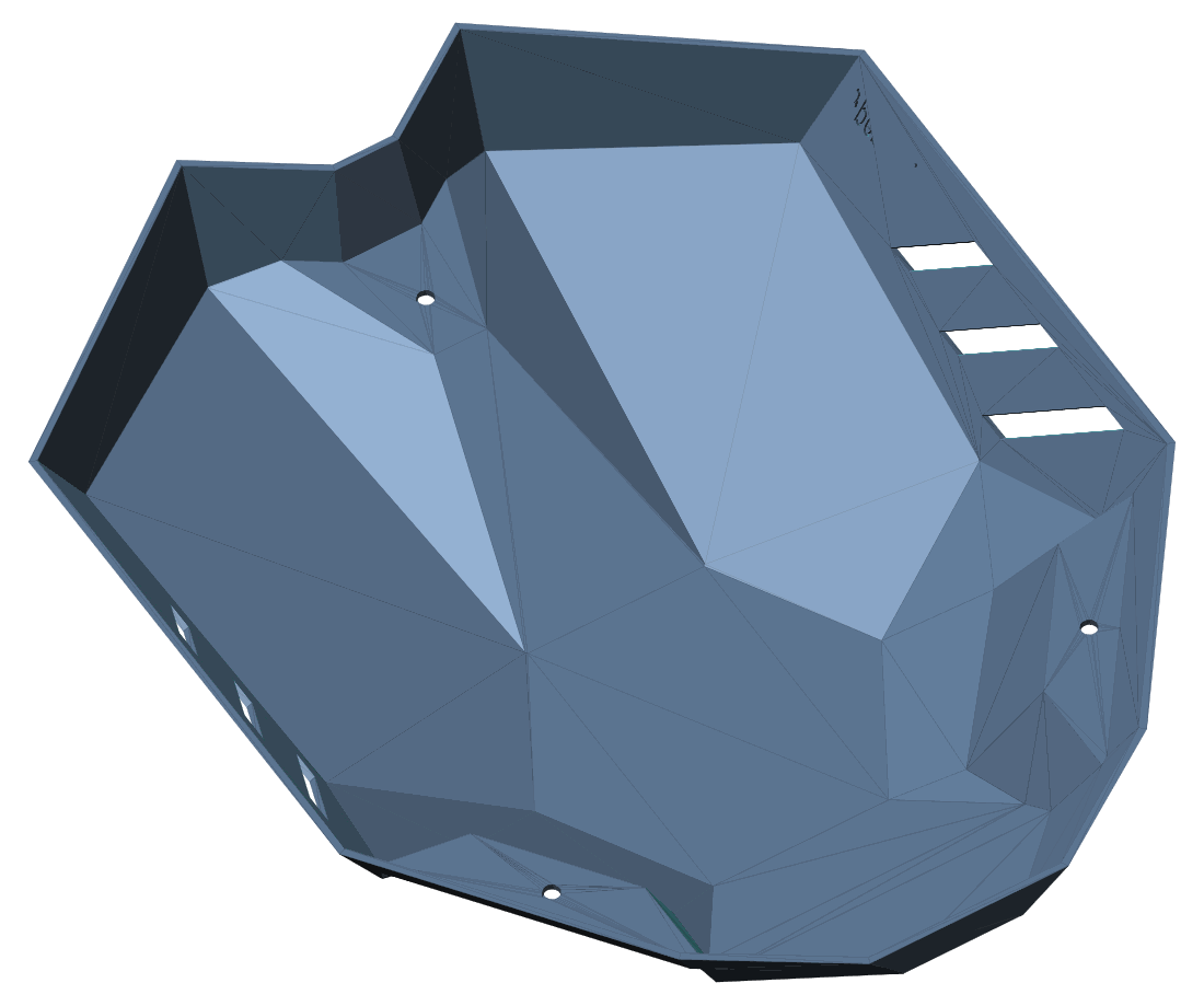
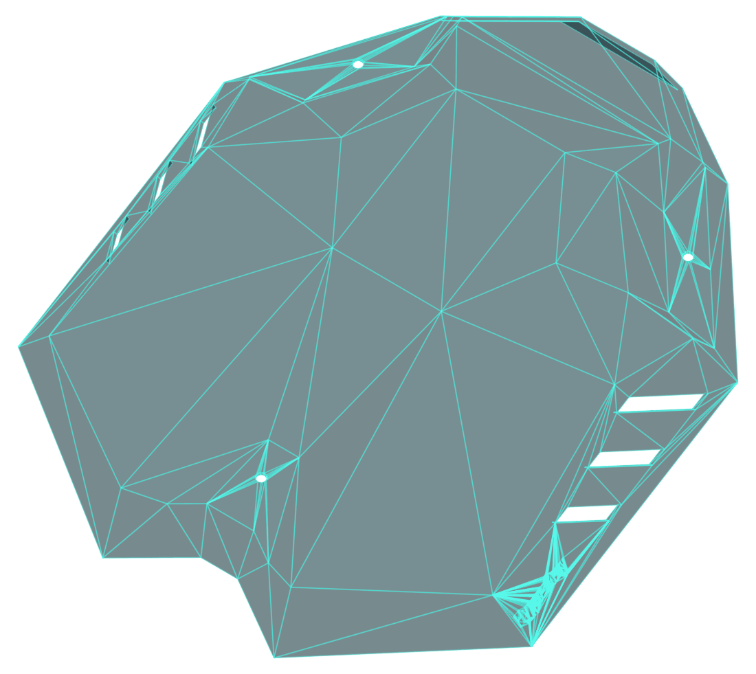

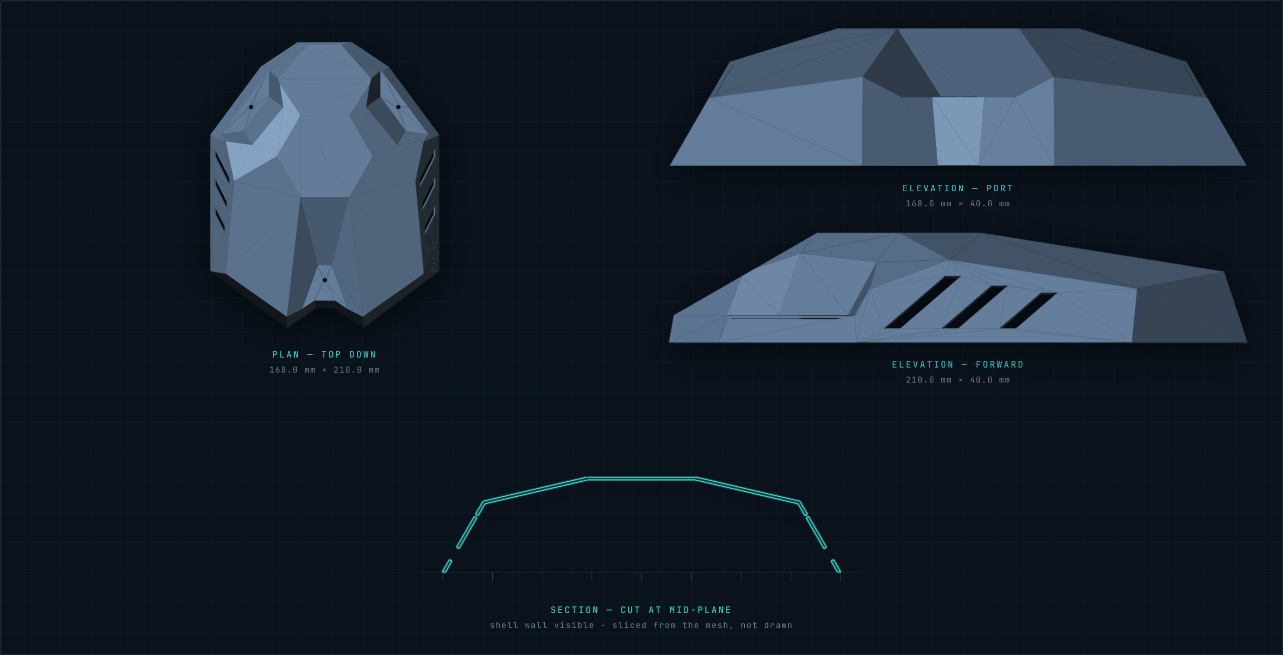
The part
- Envelope
- 168 × 210 × 40 mm
- Geometry
- 3,934 triangles, binary STL
- Verified
- Calipers, against the shipped file
01 Every curve carries its provenance
The number has a source.
Nothing on this site is asserted without a label. Each figure is measured, calculated, modelled or referenced, and each one traces back through the chain that produced it to a piece of published physics or a bench reading. Follow any stage below.
Given
Derived
Decided
02 The adaptation is not a lookup table
The pulse is a decision.
The solver scores every candidate pulse against the current acoustic link budget and takes the widest sweep that still clears its margin. Move the water and watch the candidates re-score. The frequency changes because the scores changed — there is no turbidity-to-frequency table anywhere in this project.
— NTU
51000 NTU
Temperature, salinity and depth are held at the operating point the published sweep was run at, so this reproduces that table exactly.
Current water
- Temp
- — °C
- Salinity
- — ppt
- Turbidity
- — NTU
- Depth
- — m
Current solution
- fC
- — kHz
- Bandwidth
- — kHz
- Resolution
- — mm
- Margin
- — dB
fC kHz B kHz Margin dB Res mm Verdict
The candidate table is computed in the browser.
A candidate must clear the detection threshold plus the margin this water demands — — dB in total. The solver takes the widest surviving sweep, not the strongest echo, because bandwidth is what buys range resolution.
Why
- Spreading
- — dB
- Absorption
- — dB
- Scattering
- — dB
—
Frequency falls a long way. Usable range does not — the solver is spending resolution to keep the link closed, which is the trade the whole payload exists to make.
03 It runs with nothing attached
The vehicle carries the loop.
Sensing, estimation, waveform selection, synthesis, transmission and correlation all happen on the payload, between one ping and the next. There is no server in the path, no pairing step and no surface link — which is the only arrangement that works on a deck with no connectivity and a vehicle already under.
- 01 Environment the water
- 02 Sensors temp · TDS · turbidity · depth
- 03 Estimation c, α, excess
- 04 Selection the solver
- 05 DDS phase accumulator
- 06 DAC 12-bit
- 07 Conditioning reconstruction filter
- 08 Drive analog stage
- 09 Transducer pressure wave
- 10 Echo the return
- 11 Processing matched filter
- 12 Telemetry to the deck app
- Sample
- Estimate
- Solve
- Synthesise
- Transmit
- Receive
- Correlate
Shown in execution order.
04 The loop is closed, and visible
The model can be wrong.
A prediction that cannot be checked is an opinion. The payload compares the echo it predicted against the echo it received and carries the difference into the next decision as a correction term. That term is implemented and you can drive it below — the measurement that will feed it is the next rung on the validation ladder.
- 01 Measure the water
- 02 Model predict the echo
- 03 Transmit the chosen pulse
- 04 Receive what came back
- 05 Compare predicted against received
- 06 Retune carry the error forward
Implemented Correction term · implemented
decide() takes a correction term. Raising it makes the solver assume a worse link than its own physics predicts, and re-solve against that. Which way the answer moves is the model's to decide, not ours — that is running below.
Rung 05 Signal exists in water
The same test in a tank. This is where absorption and scattering start behaving like the model says they should — or do not.
— dB
0 dB12 dB
Model on its own — kHz · —
Next decision, corrected — kHz · —
Range resolution — was —
—